1. Introduction
Machine learning models are getting larger and larger, and these larger models tend to perform better. However, these larger models have high memory requirements just to load them into memory. Consumer hardware doesn’t have a huge amount of memory to load these large models. Model compression is a technique used to compress large models into smaller ones at the expense of small to negligible inaccuracies. The compressed models can be optimized to run on consumer hardware and can make use of NPUs for high performance.
2. Model Compression
Model compression provides three ways to compress models:
Quantization - Quantization is a technique where we store the parameters of the models in lower precision. For example: FP32 to INT8.
Knowledge Distillation - In Knowledge Distillation, the original model (Instructor) transfers its knowledge to a smaller model (Student model). The premise is that while training, the larger model learns various important aspects that can be represented using smaller number of parameters in the student model.
Pruning - In Pruning, we remove the connections in the model that do not contribute much to the model’s output. This results in a sparse and computationally efficient model.

3. Data Types used in ML
Generally, the integer and floating point data types are used for ML models.
3.1. Integers
Integers can be stored as either unsigned or signed integers to represent positive and negative values, respectively. For signed integers, the 2’s complement representation is used.

The range of unsigned and signed integers differs because a sign bit is used to represent the sign of the integer.
- $n$-bit unsigned Integer: $[0, 2^{n}-1]$, For 8bit: $[0,255]$
- $n$-bit signed Integer: $[-2^{n-1}, 2^{n-1}-1]$, For 8 bit: $[-128, 127]$
3.2. Floating Point
Floating point numbers are numbers that have fractional parts as well. In computers, floating point numbers are first normalized to the form below and stored using three components:
$$ \text{Real Number} = (-1)^{\text{S}} \times 2^{E+B} \times 1.M $$
Example: $$ 1272.125 = (-1)^0 \times 2^{10+127} \times 1.0011111000001 $$
- Sign Bit (S): Represents the sign of the number.
- Exponent (E): Represents the range of the number.
- Mantissa (M): Represents the precision of the number, also called fraction bits.
- Bias (B): A bias constant is used to split the exponent range to cover both positive and negative exponents.
FP32, FP16, BF16, and FP8 are the common floating point data types used in machine learning. The different variants of floating point numbers reserve different bits for the exponent and fraction. There is a trade-off between precision and range. More precision bits allow storing smaller numbers but can’t store numbers with a large range, and vice versa.
| Data Type | Exponent Bits (Range) | Fraction Bits (Precision) | Precision | Range |
|---|---|---|---|---|
| FP32 | 8 | 23 | Best | Best |
| FP16 | 5 | 10 | Better | Good |
| BF16 | 8 | 7 | Good | Better |
| FP8 | 5 | 2 | Bad | Good |
We can downcast higher bit floating point numbers to lower bit floating point numbers. However, there are a few pros and cons to this approach.
Pros:
- Downcasting floating point numbers results in lower memory requirements for inference and storage.
- Increased computation speed, as hardware is faster when performing operations with FP16 compared to FP32.
Cons:
- Loss of precision due to fewer bits being available for representing the same number in lower precision floating point.
4. Linear Quantization
We will focus on linear quantization in this post. The quantization techniques are modality agnostic and can be used for any type of model, whether it is text, voice, image, etc. The techniques we are going to study in this blog fall into the post-training quantization (PTQ) category, as they are applied once the model is trained. There are two types of linear quantization:
- Symmetric Quantization - which only has a scale.
- Asymmetric Quantization - which has a scale and zero-point.
4.1 What can be Quantized?
We can quantize the:
- Weights ($w$, $b$): The parameters of the neural networks.
- Activations ($a$): The values that propagate through the network.
$$a = g(w \cdot x + b)$$
4.2. Asymmetric Quantization
Asymmetric Quantization is a linear mapping that maps a higher range to a lower range. It has two parameters: scale and zero-point.
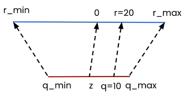
4.2.1. Formula for Asymmetric Quantization:
$$q = \text{int}(\text{round}(\frac{r}{s}) + z) \tag{1} $$
where $r$ is the original value, $s$ is the scale in unquantized range, $q$ is the quantized value, and $z$ is the zero-point in quantized-space.
4.2.2. Formula for Asymmetric De-quantization:
By rearranging the previous equation for $r$, we get: $$ r = s(q - z) \tag{2} $$
4.2.3. Determining Scale and Zero-Point
For the optimal values of scale and zero-point, $r_{min}$ should be mapped to $q_{min}$ and $r_{max}$ should be mapped to ${q_{max}}$. Therefore at extreme points, we have below equations.
$$ r_{min} = s(q_{min} - z) $$ $$ r_{max} = s(q_{max} - z) $$
For scale, we can subtract these equations and re-arrange for $s$.
$$ s = \frac{r_{max} - r_{min}}{q_{max} - q_{min}} $$
For zero-point, we can rearange the above equation for $z$
$$z = \text{int}(\text{round}(q_{min} - \frac{r_{min}}{s}))$$
4.2.4. Example of Asymmetric Quantization
Let’s convert an FP32 tensor to INT8.

$$[ r_{min}, r_{max} ] = [ -184, 728.6 ]$$ $$[ q_{min}, q_{max} ] = [ -128, 127 ]$$
Let’s calculate the scale and zero-point.
$$s = \frac{728.6 - (-184)}{127 - (-128)} = 3.5788$$ $$z = \text{int}(\text{round}(-128 - \frac{-184}{3.5788})) = \text{int}(-77.0) = -77$$
Using the calculated scale and zero-point from above in equations (1) and (2), we get the following quantized and unquantized tensors.

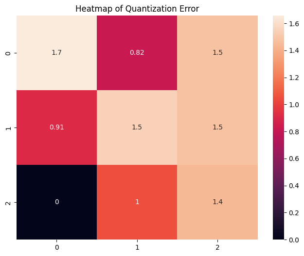
Quantization is not lossless, and hence some information is lost during the conversion process. The image below shows the quantization error heatmap.